data-science-I
Things to talk about?
- Distance Metrics ?
This post is in progress.
Categorical variable is called qualitative variable/predictors and numerical variables is called quantitative variables.
Common steps for the data cleaning:
Better the data, fancier the algorithm will be
- memory optimization of numerical feature
int64 -> int16, int32 - Duplicate observation removal
- Filter outlier
- num feature: use box/distribution plot, either drop them or replace them with mean or another corner element(upper-bound)
prefered - cat feature: create a spearate category for outlier or fill null. Also can use new feature, which represent outlier
- num feature: use box/distribution plot, either drop them or replace them with mean or another corner element(upper-bound)
- handle missing value using
inter-quartile range - Fo text data, we have following step:
- Convert all words to Lower Case
- contraction mapping
isn't -> is not. - Extra Space removal
- Punctualtion removal
- Digit and other special character removal.
- clean html markup or other sort of chracter
- Type conversion.
integer -> categoryfor cat feature
- Standardize/Normalization
- Feature transformation
X -> logX
IQR:
The IQR approximates the amount of spread in the middle half of the data that week. Step to find iqr is:
- sort the data
- create two buckets of data
- even size: divided data is of odd size
- odd size : divided data is of even size
- Pick the median from each bucket and take the diff
Missing Data Handling:
There are 3 types of missing data cases:
- Completely missing at random
- Missing at random
- Not missing at random
Here is the graph, which tells all about
biashappens, in these three cases: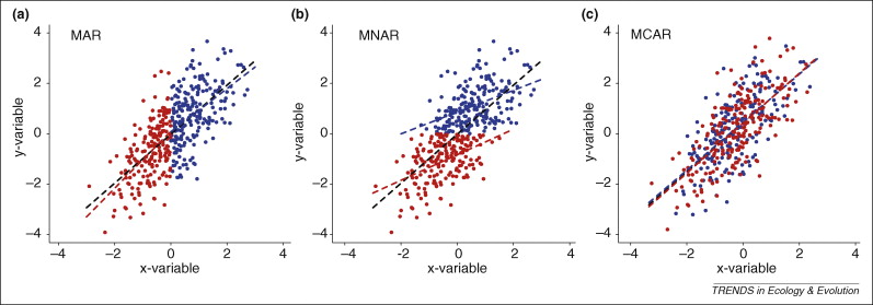 Source: Nakagawa & Freckleton (2008)
To test these cases:
- We can partition data into two big chunks and compute the
t-testfor both sepeartely.- If
t-valueis same, then it isCMAR. - Else it may be the case of
MARorNMAR
- If
Methods for missing value imputation:
- Mean, Mode, Median imputation
- KNN based, we can take average of its
knearest neighbours (not very good for higher dimensional data)- Euclidean, Manhattan, cosine similarity
- Hamming Distance, jaccard(very good for sparse data)
- Tree based Imputation
- EM (Iterative approach)
- Linear Regression based
- assume missing-value attribute as depeendent variable and all other variable as independent
- predict the batch of missing value and include them as well for training
- repeat till converge
it add linearity, make worse this model
- Mice [Multiple imputation by chained equation]:
- Assume feature/predictor with missing value as dependent variable and rest of them as independent variable.
- Fit any predictive modelling algo such as linear regression and predict for the missing value
Sampling Techniques:
To model the bahaviour of population, we need a good strategy to choose sample, which can describe the model bahaiour.
We can’t deal with entire population, better is to chose some sample which will have same empirircal mean as that of entire population mean
Exp: when we are building some application or running some experiment, we never have the population sample, we have subset of that population. Now our objective is to approximate the behaviour of population, using emperical observation. So our sampling helps here.
Bootstrap sampling is very important in this context. As it is proved that if we build model using bootstrap sampling and run this experiment a large number of times, its avg emperical mean approx equal to population mean.
Sampling can be categorize in two buckets in broad ways:
- Probability based sampling
- allot some propbability to sample, can be weighted or uniform(mostly)
- weighted sampling, acc to user experience. For example, in a servey of maedical diagnose, an doctor servey will be more important than patient’s response.
- Random Sampling
- Staratified Sampling
- divide the population into groups/strata and then use random sampling on each group 3. Bootstrap sampling
- random sampling with replacment
- an average bootstrap sample contains
63.2%of the original observations and omits36.8%. - The probability that a particular observation is not chosen from a set of n observations is
1 - 1/nand for collecting thensamples, it becomes(1 - 1/n)^n. - proof: As
n → ∞ of (1 - 1/n)^n is 1/e. Therefore, when n is large, the probability that an observation is not chosen is approximately 1/e ≈0.368. very importantto build decorrelated model inbagging
- Non-Probability based
- Convenience Sampling
- choose, whatever you can find
- biased
- not efficient
- poor representation of population
- Quota sampling
- order based sampling
- select some random number and then choose k samples in ascending/some order
- Biased
- poor representation
- Convenience Sampling
Basic Step of ML practising:
- Explore the data
- draw
histogram,cross-plotand so on understand the data distribution
- draw
- Feature Engineering
- Come up with hypothesis (with assumption) and prove your hypothesis
- Color can be important on buying second hand car, It is better to embedded color, instead of feeding raw data of images as it is.
- In text data-set, length, average and other statistics of sentence can be another features
- In tree based model, this statistics can be helpful
- Log(x), log(1 + x), fit poisson distribution for counting variable
- For large categorical in a feature, mean encoding is very helpful, also it helps in converge fast. First check its distribution or distribution before and after encoding
- Fit a model
Stacking (stack net)
- It is a meta modelling approach.
- In the base leevl, we train week learner and then their prediction is used by another models, to get final prediction.
- It is simply a NN model, where each node is replaced by one model.
Process:
- Split the adta in K parts
- train weak learner on each K-1 parts and holdout one part for prediction for each weak learner
- Algorithm steps with exp:
- We split the dataset in 4 parts.
- Now, train first weak learner on 1,2,3 and predict on 4th.
- Train 2nd weak learner on 1,2,4 and predict on 3rd.
- repeat on
- Now, we have prediction of eavh learner on separate hold-out and after combining all, we get prediction on entire data-set.
Data-Leakage
- data-leakage make model to learn something other than what we intended.
- produce bias in model
- If we have information or feature in training data-set, that is outside from training data-set or that features has not any coorelation with the training data distribution, that is data-leakage
How do we induce data-leakage (generally)?: While building model, if we use entire data (train + test) for standardization which will know the entire distribution. Whereas our aim is to learn that distribution by training our model only trainining data-set.
Use standarization o training data-set and while testing normalize the test data with the same parameters used in training time.
Cross Validation
We generally, split our data-set into training and testing. Further from training data-set, we take some part for validation. This is classical setting. We use K-Fold validation strategy to obtain unbiased estimate of the performance, i.e. sum of all fold’s prediction / K
Noe that this K-Fold validation considers on training data
Nested Validation
This is more robust method, Especially in time-series dataset, where data-leakage generally occurs and affect the model performance by an enormous amount.
The idea is that there are two loops, One is outer loop, same as classical validation step and another is inner loop, where futher training data in one step of K-Fold is divided into training and validation and The 1-Fold, which is hold for validation in outer loop, act as testing dataset.
Using nested cross-validation, we train K-models with different paraameters, and each model use grid serach to find the optimal parameters. If our model is stable, then each model will have same hyper-parameyters in the end.
Why is Cross-Validation Different with Time Series?
When dealing with time series data, traditional cross-validation (like k-fold) should not be used for two reasons:
- Temporal Dependencies
- Arbitrary choice of Test data-set
Nested CV method
- Predict Second half
- Choose any random test set and on remaining data-set, main training and validation with temporal relation
- Not much robust, because opf random test-set selection.
- Forward chaining Maintain temporal relation between all three train, validation and test set.
- For example, we have data for 10 days.
- train on 1st day, validate on 2nd and test on else
- train on first-two, validate on third and test on else
- repeat. This method produces many different train/test splits and the error on each split is averaged in order to compute a robust estimate of the model error.
Feature Selection [src-analytics-vidya]:
- Filter Methods
- Wrapper Methods
- Embedded Methods
- Difference between Filter and Wrapper methods
Filter Methods.
-
Pearson’s Correlation: It is used as a measure for quantifying linear dependence between two continuous variables X and Y. Its value varies from -1 to +1. -
LDA: Linear discriminant analysis is used to find a linear combination of features that characterizes or separates two or more classes (or levels) of a categorical variable. -
Chi-Square: It is a is a statistical test applied to the groups of categorical features to evaluate the likelihood of correlation or association between them using their frequency distribution.
NOTE: Filter Methods does not remove multicollinearity.
wrapper methods:
Here, we try to use a subset of features and train a model using them. Based on the inferences that we draw from the previous model, we decide to add or remove features from your subset.
- This is computationally very expensive.
Methods:
- forward feature selection
- we start with having no feature in the model. At each iteration, we keep adding the feature which best improves our model
- backward feature elimination
- we start with all the features and removes the least significant feature at each iteration which improves the performance of the model
- recursive feature elimination
- It is a greedy optimization algorithm which aims to find the best performing feature subset.
- It repeatedly creates models and keeps aside the best or the worst performing feature at each iteration.
- It constructs the next model with the left features until all the features are exhausted.
- It then ranks the features based on the order of their elimination.
- It is a greedy optimization algorithm which aims to find the best performing feature subset.
Difference between Filter and Wrapper methods
The main differences between the filter and wrapper methods for feature selection are:
- Filter methods measure the relevance of features by their correlation with dependent variable while wrapper methods measure the usefulness of a subset of feature by actually training a model on it.
- Filter methods are much faster compared to wrapper methods as they do not involve training the models. On the other hand, wrapper methods are computationally very expensive as well.
- Filter methods use statistical methods for evaluation of a subset of features while wrapper methods use cross validation.
- Filter methods might fail to find the best subset of features in many occasions but wrapper methods can always provide the best subset of features.
- Using the subset of features from the wrapper methods make the model
more prone to overfittingas compared to using subset of features from the filter methods
Afterward, post is in progress.
Feature SelectionMore-Info
1) Feature selection with correlation and random forest classification
correlation map
f,ax = plt.subplots(figsize=(18, 18))
sns.heatmap(x.corr(), annot=True, linewidths=.5, fmt= '.1f',ax=ax)
using this coorelation map, we select some of the feature and check our algo pred rate.
from sklearn.model_selection import train_test_split
from sklearn.ensemble import RandomForestClassifier
from sklearn.metrics import f1_score,confusion_matrix
from sklearn.metrics import accuracy_score

# split data train 70 % and test 30 %
x_train, x_test, y_train, y_test = train_test_split(x_1, y, test_size=0.3, random_state=42)

#random forest classifier with n_estimators=10 (default)
clf_rf = RandomForestClassifier(random_state=43)
clr_rf = clf_rf.fit(x_train,y_train)

ac = accuracy_score(y_test,clf_rf.predict(x_test))
print('Accuracy is: ',ac)
cm = confusion_matrix(y_test,clf_rf.predict(x_test))
sns.heatmap(cm,annot=True,fmt="d")

Accuracy is:  0.9532163742690059
2) Univariate feature selection and random forest classification In univariate feature selection, we will use SelectKBest that removes all but the k highest scoring features
from sklearn.feature_selection import SelectKBest
from sklearn.feature_selection import chi2
# find best scored 5 features
select_feature = SelectKBest(chi2, k=5).fit(x_train, y_train)

print('Score list:', select_feature.scores_)
print('Feature list:', x_train.columns)
Using this selction score, we obtain the top k feature, using transform function
x_train_2 = select_feature.transform(x_train)
x_test_2 = select_feature.transform(x_test)
#random forest classifier with n_estimators=10 (default)
clf_rf_2 = RandomForestClassifier()
clr_rf_2 = clf_rf_2.fit(x_train_2,y_train)
ac_2 = accuracy_score(y_test,clf_rf_2.predict(x_test_2))
print('Accuracy is: ',ac_2)
cm_2 = confusion_matrix(y_test,clf_rf_2.predict(x_test_2))
sns.heatmap(cm_2,annot=True,fmt="d")

Accuracy is:  0.9590643274853801
3) Recursive feature elimination (RFE) with random forest Basically, it uses one of the classification methods (random forest in our example), assign weights to each of features. Whose absolute weights are the smallest are pruned from the current set features. That procedure is recursively repeated on the pruned set until the desired number of features
from sklearn.feature_selection import RFE
# Create the RFE object and rank each pixel
clf_rf_3 = RandomForestClassifier()
rfe = RFE(estimator=clf_rf_3, n_features_to_select=5, step=1)
rfe = rfe.fit(x_train, y_train)

print('Chosen best 5 feature by rfe:',x_train.columns[rfe.support_])

Chosen best 5 feature by rfe: Index(['area_mean', 'concavity_mean', 'area_se', 'concavity_worst',
       'symmetry_worst'],
      dtype='object')
In this method, we select the no of feature, what if we select less no of feature than which can increase acc much greater than this.
4) Recursive feature elimination with cross validation and random forest classification
Now we will not only find best features but we also find how many features do we need for best accuracy.
from sklearn.feature_selection import RFECV

# The "accuracy" scoring is proportional to the number of correct classifications
clf_rf_4 = RandomForestClassifier()
rfecv = RFECV(estimator=clf_rf_4, step=1, cv=5,scoring='accuracy')   #5-fold cross-validation
rfecv = rfecv.fit(x_train, y_train)

print('Optimal number of features :', rfecv.n_features_)
print('Best features :', x_train.columns[rfecv.support_])

# Optimal number of featu<!-- res : 14
# Best features : Index(['te -->xture_mean'....]

plt.plot(range(1, len(rfecv.grid_scores_) + 1), rfecv.grid_scores_)
5) Tree based feature selection and random forest classification
Random forest choose randomly at each iteration, therefore sequence of feature importance list can change.
clf_rf_5 = RandomForestClassifier()
clr_rf_5 = clf_rf_5.fit(x_train,y_train)
importances = clr_rf_5.feature_importances_
std = np.std([tree.feature_importances_ for tree in clf_rf.estimators_],
             axis=0)
indices = np.argsort(importances)[::-1]

# Print the feature ranking
print("Feature ranking:")

for f in range(x_train.shape[1]):
    print("%d. feature %d (%f)" % (f + 1, indices[f], importances[indices[f]]))

# Plot the feature importances of the forest

plt.figure(1, figsize=(14, 13))
plt.title("Feature importances")
plt.bar(range(x_train.shape[1]), importances[indices],
       color="g", yerr=std[indices], align="center")
plt.xticks(range(x_train.shape[1]), x_train.columns[indices],rotation=90)
plt.xlim([-1, x_train.shape[1]])
plt.show()

Feature ranking:
1. feature 1 (0.213700) ....
Cat var: Qualitive variable Num var: Quantitative Var
t-statistics: Final the coeeficient of feature in model and also find the std dev error and t-stat = (coeff/std-dev error)